Mikrobiomo 16S Analysis Example Report
Content
I. Overview
facultative_report.general_vision_p1
In this case, amplicon sequencing is performed using the Illumina platform following paired-end algorithm analysis.
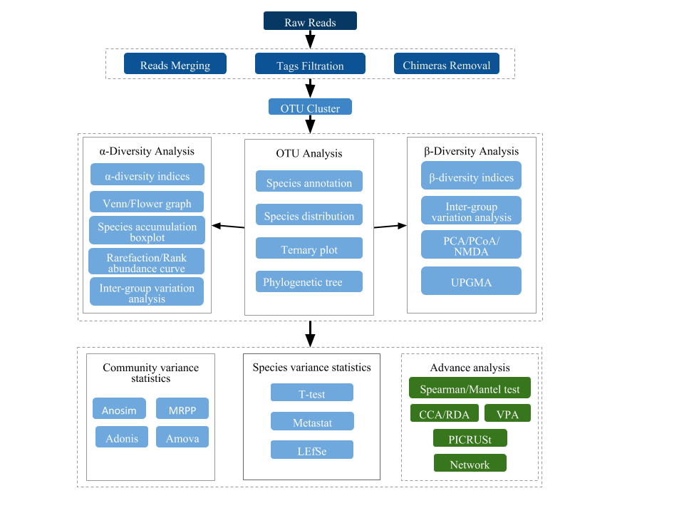
II. Workflow
1 Preparation and Sequencing
From raw DNA samples to final data, each step (including sample testing, PCR, library preparation and sequencing) influences the quality of the data and this, in turn, directly impacts the results of the analysis. To maintain data reliability, quality control (QC) is performed at each step of the procedure. Thus, the workflow is as follows:

2 Data Analysis and Procedures
For accuracy of sequencing analysis, raw data is merged and filtered to clean data. The effective data is used to make annotations of groups and species of Operational Taxonomic Units (OTUs) for the respective sequence of each of them. Therefore, relative species distribution, evenness, and abundance can be analyzed with alpha diversity, beta diversity, or the Venn or Flower diagram (Graph et al.). Furthermore, both OTU selection and phylogenetic tree taxonomic assignment construction through post statistical analysis (PCoA, PCA and NMDS) explain differences in microbial community construction between samples or groups. Statistical methods such as T-test, MetaStat, LEfSe, Anosim, and MRPP could test the importance of community composition and structure differences between groups. Meanwhile, the analysis result combines CCA/RDA to explore the main environmental factors. The data analysis workflow is shown below:
Notes: If the number of samples is less than 3, Beta diversity analysis, microbial community significance test, build difference between groups, and environmental association analysis cannot continue. The significance test of the community construction difference between groups and the environmental association analysis cannot proceed without clustering, or in case the repetition is less than 3. The environmental association analysis needs the data of the environmental factor that customers offer.
III. Results
1 Sequencing Data Processing
The resulting amplicon has been sequenced using the Illumina platform and features an even end of 250bp raw reads (RAW PE), then assembled and pretreated to clean labels. Chimeric sequences in the clean tags were detected and removed to finally obtain the effective tags. The data output is shown in table 1.
Table 1. Statistic QC
Notes: Raw PE ≡ Raw Reads; Raw Tags ≡ Raw Tags (raw PE merger); Clean Tags ≡ Clean tags after filtering; Effective Tags ≡ Effective tags after filtering out chimeras; Base (nt) ≡ Number of effective tag bases; AvgLen ≡ Average length of effective labels; Q20 and Q30 ≡ Percentage of base whose quality is higher than 20 and 30, respectively; GC (%) ≡ GC content in effective labels; Effective (%) ≡ Percentage of effective tags in the raw reads.
2 OTU Analysis and Species Annotation
To analyze species diversity in each sample, all effective tags were grouped by 97% DNA sequence similarity in OTUs (Operating Taxonomic Units).
2.1 OTU Identification and Annotation
2.1.1 Statistical Analysis Annotation
During the construction of the OTUs, basic information was collected from different samples, such as effective tag data, low frequency tag data, and tag annotation data. The statistical data set is shown below in figure 2.1.1 (To see the full size image, click here).
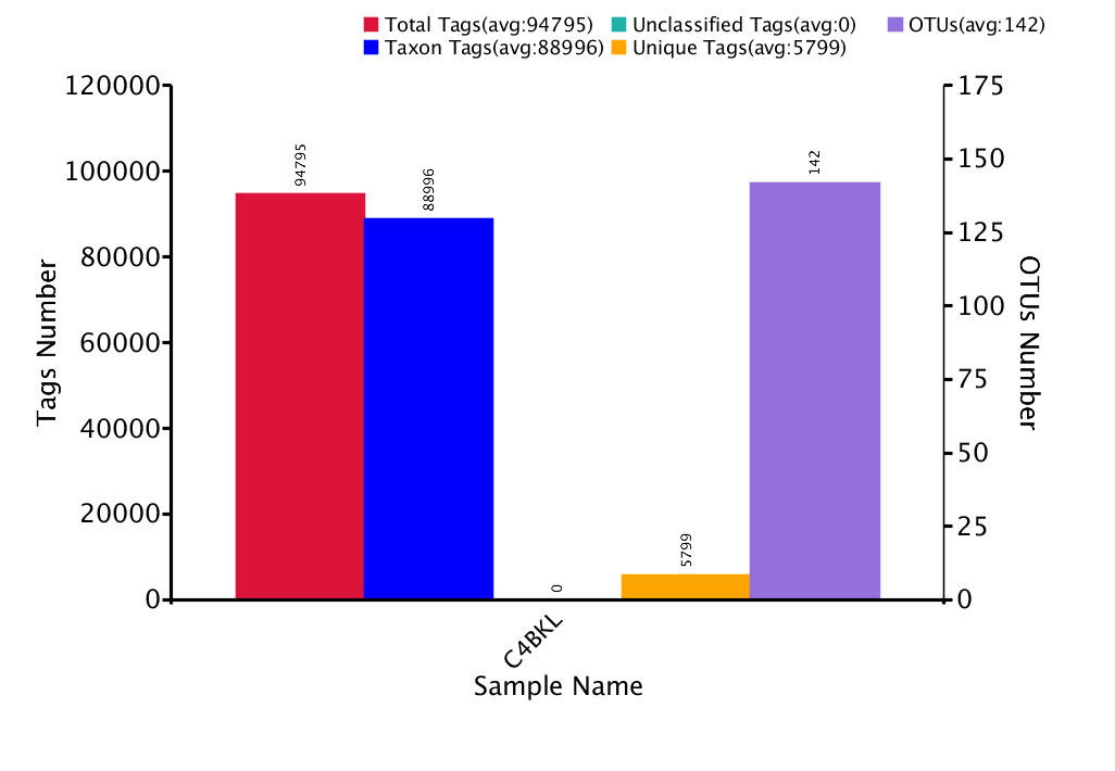
Figure 2.1.1 Statistical analysis of the labels and number of OTUs of each sample
Notes Graph 1. Statistical Analysis: Total reads ≡ Total reads (red bars); Total Merged ≡ Merged Readings or Contings (yellow bars); Total Denoised ≡ Unannotated readings or background noise (grey bars); Total Filtered ≡ Readings with a Quality Score (Q) greater than 30 (purple bars); Total Non–Chimeric ≡ Reads without chimeras (blue bars). Notes Graph 2. Number of OTUs per Sample: The red bars refer to the number of Operational Taxonomic Units (OTUs) present in the sample M1.
2.1.2 Interactive Species Annotation View
The heat map displays an interactive view of the species composition and abundance between different samples on the live web page Click here . An example image shows the following:
Figure 2.1.2 Example heatmap showing taxonomy mapping for each OTU.
Notes: Clicking the "Sample ID" button displays counts colored according to the percentage contribution of each OTU to the total count of OTUs in a sample (blue ≡ low percentage; red ≡ high percentage). Switching to the “Taxonomy” button shows the taxonomy in detail. For more details, click here for details..
2.1.3 Taxonomy Tree:
Specific species (showing top 10 genera in high relative abundance by default) were selected to make the taxonomy tree[4] using independent R&D software.The tree of taxonomy in a single sample is shown in Figure 2.1.3-1. click).
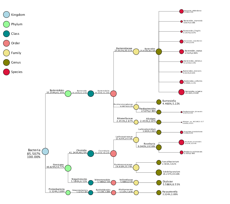
Figure 2.1.3-1 Taxonomy Tree in Unique Sample.
Notes: The different colors represent different taxonomic ranges. The size of the circles represents the relative abundance of species. The first number below the taxonomic name represents the percentage in the entire taxon, while the second number represents the percentage in the selected taxon.
2.1.4 Krona Display
KRONA [5] visually displays the result of the species annotation analysis. Circles from inside to outside represent different taxonomic ranges, and sector area means the respective proportion of different OTU annotation results.
Figure 2.1.4 Krona Display
2.2 Species Composition Analysis
2.2.1 Relative abundance of taxa
The top 10 taxa in the different taxonomic ranges were selected to form the relative abundance distribution histogram. The distribution in phylum was shown as follows (To see the full size image, please click here):
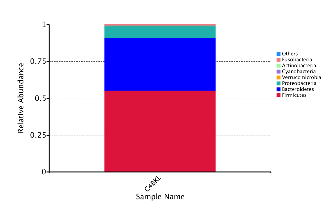
Figure 2.2.1 facultative_report.ab_relative_filo
Notes: Plotted by "Relative Abundance" on the Y-axis and "Sample Names" on the X-axis. "Other" represents a total relative abundance of all other phyla in addition to the top 10 phyla.
2.2.2 The Evolutionary Tree in Genus.
The top 100 genera were selected and the evolutionary tree drawn using the aligned representative sequences. The relative abundance of each genus was also shown across the genus in Figure 2.2.2:
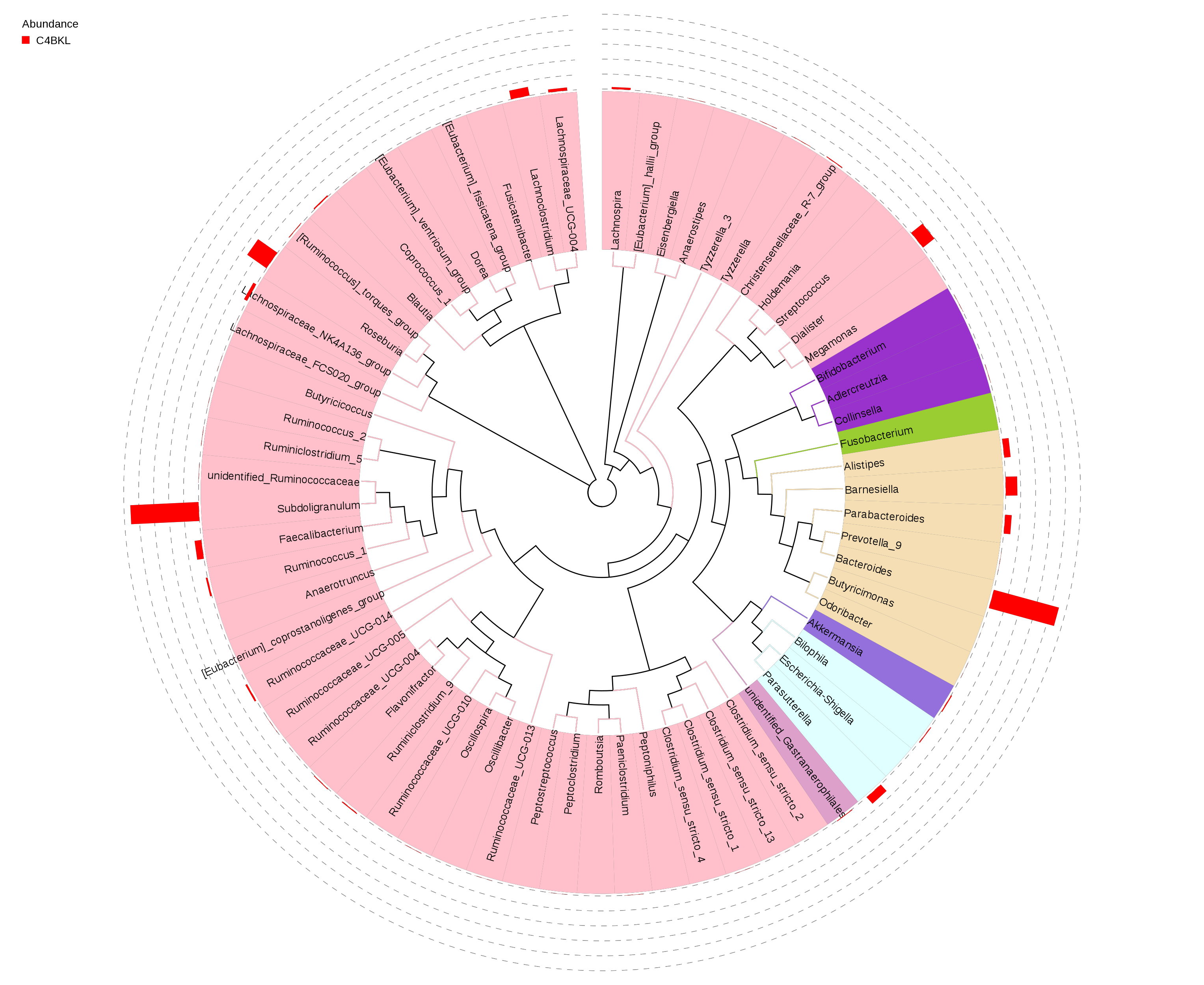
Figure 2.2.2 The Evolutionary Tree in Gender
Notes: The different colors of the branches represent different phyla. The relative abundance of each genus in each group was shown outside the circle and the different colors represent different groups.
3 Alpha Diversity Analysis
Alpha diversity is widely used to assess microbial diversity within a community [6], including species accumulation box plots, species diversity curves, and indices of statistical analysis.
3.1 Alpha Diversity Indices
Generally speaking, OTUs generated with 97% sequence identity are considered homologous in species. The statistical indices of alpha diversity when the clustering threshold is 97% are summarized below: (Number of reads chosen for normalization: cutoff = 88996. The meaning of each alpha diversity index is listed in Method-Data Analysis- 3 Alpha diversity analysis).
Table 3.1 Alpha Diversity Index Statistics
3.2 Species Diversity Curve
Rarefaction curves and rank abundance curves are widely used to indicate the biodiversity of samples. The rarefaction curve is created by randomly selecting a certain amount of sequencing data from the samples and then counting the number of species they represent. If the curve is steep, many species remain to be discovered. If the curve becomes flatter, a credible number of samples have been taken, meaning that only the rare species remain to be sampled.
The range of abundance curve is used to display the relative abundance of species. It can also be used to visualize species richness and uniformity. It overcomes the deficiencies of the biodiversity indices that cannot present the role that the variables played in its evaluation[7].
Species Diversity Curve (To see the full size image please click):
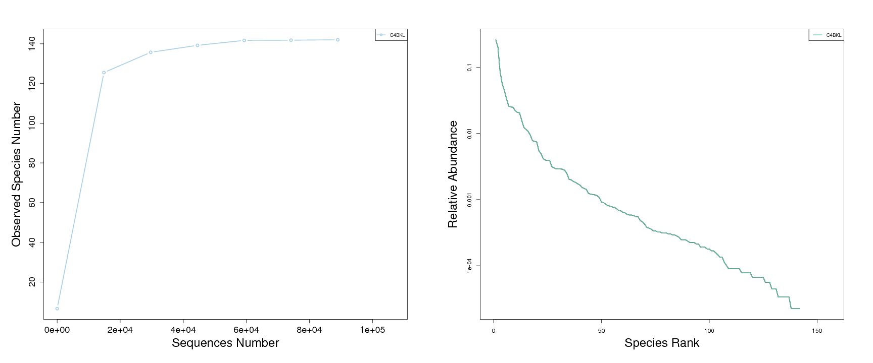
Figure 3.2-1 Rarefaction Curves Figure 3.2-2 Abundance Rank Curves
Notes: For rarefaction curves, each curve represents a sample and can be colored and shaped by each sample name provided in the mapping file. The number of sequences is on the x-axis and the number of observed OTUs is on the y-axis. For the rank-abundance curves, each curve represents a single sample, plotted by the relative abundance of OTUs on the y-axis and the rank of OTU abundance on the X-axis, which can be colored and shaped by each sample name provided in the mapping file.
4 Data Processing
16S rDNA (18S rDNA, ITS) amplicon sequencing is widely used for comparison of microbial communities between samples from various natural or endozoic environments such as soil, water, host gut, etc.
First, the results of the OTU group and species annotation are summarized into a file where the labels are grouped with 97% identity. All rendered tags for each OTU are listed in an artifact, noted, and collected. On the other hand, the abundance of species was obtained through two ways: the absolute abundance of species in different taxonomic ranges and after normalization; and the relative abundance of each sample after normalization. The data is summarized for subsequent analysis of alpha diversity and beta diversity, the results of which allow the visualization of the species composition of various samples, as well as those species in question or that differ markedly between samples (or groups).
The distribution of dominant species among the samples is displayed in a bar graph and in a profile table identifying the notably predominant species quickly. Subsequently, the abundance analysis and the difference tests are performed.
Six different alpha diversity indices are included in the sample complexity results (Observed Species, Asset Coverage, Chao1, ACE, Shannon, Simpson).
As for comparing microbial community differences between samples, the Unifrac distance between pairwise samples is displayed as a heat map to measure and view the degree of dissimilarity. Subsequently, this is calculated with a gradient analysis and displayed with ordination plots (PCA, PCoA, etc.). Generally, samples with a similar microbial community structure tend to be collected. The unweighted pairwise ranking with arithmetic means (UPGMA) method groups the samples based on the acquired distance matrix. From these results, the differences in complexity between samples are determined, making it possible to relate them to specific underlying biological problems. For example, UPGMA sample clustering results can be explained by considering high-abundance taxa to achieve the underlying driving factors.
When there are more than two groups, more advanced analysis could be done.
For species differences, we can use Metastats to get the importance of all species between groups and select obvious different species between groups in various taxonomic ranges (p, c, o, f, g, s) to a more detailed analysis, or choose LefSE analysis to discover statistically significant biomarkers between groups.
Anosim and MRPP analysis could be used to determine if community structure differs significantly between groups, or compare differences between groups and within groups.
NMDS analysis could be selected as a complementary method with unexpected results through PCA and PCoA, because it is based on a non-linear model (PCA and PCoA are based on a linear model), and it can offer a better explanation of nonlinear structure in ecological data sets.
For an exploratory analysis, if multiple environmental factors are involved, we could select CCA or RDA analysis to extract environmental gradients from ecological data sets, and find environmental drivers that influence the development of certain microbial communities.
Ⅳ. Methods
Sequencing Preparation
1 facultative_report.extraction_genoma
The total genome DNA of the samples was extracted using the CTAB/SDS method. DNA concentration and purity were monitored on 1% agarose gels. According to the concentration, the DNA was diluted to 1 ng/μL using sterile water.
2 Generation of Amplicons
Different regions of the 16S rRNA (16SV3, 16SV4), 18SrRNA (18SV4, 18SV9) and ITS (ITS1, ITS2) genes were amplified with a primer and a specific barcode for each of them. All PCR reactions were carried out using Phusion® High Fidelity Master Mix (New England Biolabs).
3 Quantification and qualification of PCR products
A 1:1 dilution of the PCR products and 1X loading buffer is made to load the 2% agarose gel. After finishing the electrophoresis, those samples with a size of 400-450 bp are selected for further experiments.
4 Mixing and Purification of PCR Products
PCR products were mixed in equal proportions and the mixture was purified with the Qiagen gel extraction kit (Qiagen, Germany).
Libraries generated with the NEBNext® UltraTM DNA Library Preparation Kit for Illumina and quantified via Qubit and Q-PCR are analyzed by the Illumina platform.
Information Analysis
1 Sequencing Data Processing
Paired reads were assigned to samples based on their unique barcode and truncated by chopping the barcode and primer sequence. The matched reads were merged using FLASH (V1.2.7) [8], a very fast and accurate parsing tool, which was designed to merge matched-end reads when at least some of the reads overlap to the readout generated from the opposite end of the same DNA fragment, and the splicing sequences were referred to as raw tags. Quality filtering on raw tags was performed under specific filtering conditions to obtain high quality clean tags [9] according to Qiime (V1.7.0) [10] quality control process. The tags were compared to the reference database (Gold database) using the UCHIME algorithm (UCHIME Algorithm)[11] to detect chimera sequences AND then chimera sequences were removed [12]. So finally the Effective Tags were obtained.
2 OTU Cluster and Species Annotation
Sequence analysis was performed by Uparse software (Uparse v7.0.1001)[13] using all effective tags. Sequences with ≥97% similarity were assigned to the same OTUs. The representative sequence of each OTU was examined for further annotation. For each representative sequence, Mothur software was performed against the SILVA SSU rRNA database[14] for species annotation in each taxonomic range (Threshold: 0.8~1).[ 15] (kingdom, phylum, class, order, family, genus, species). To obtain the phylogenetic relationship of all representative OTU sequences, MUSCLE [16](Version 3.8.31) can quickly compare multiple sequences. OTU abundance information was normalized using a sequence number standard corresponding to the sample with the fewest number of sequences. Further analyzes of alpha diversity and beta diversity were performed based on this normalized data output.
3 Alpha Diversity
Alpha diversity is applied in the analysis of the complexity of the diversity of species for a sample through 6 indices, which include Species observed, Chao1, Shannon, Simpson, ACE, Good coverage. All these indices in our samples were calculated with QIIME (Version 1.7.0) and displayed with R software (Version 2.15.3).
Alpha Diversity Indices
Community Richness Indices:
Chao - the Chao1 estimator
ACE - the ACE estimator
Community Diversity Indexes:
Shannon - The Shannon Index
Simpson - The Simpson Index
facultative_report.depth_sequencing_index
Coverage - the Good's coverage
The Phylogenetic Diversity Index:
PD_whole_tree - PD_whole_tree index
4 Beta diversity
Beta diversity analysis was used to assess sample differences in species complexity. Weighted and unweighted unifrac beta diversity was calculated using QIIME software (Version 1.7.0). Cluster analysis was preceded by principal component analysis (PCA), which was applied to reduce the dimension of the original variables using the FactoMineR package and the ggplot2 package in R software (Version 2.15.3). Principal coordinate analysis (PCoA) was performed to obtain principal coordinates and visualize complex multidimensional data. A weighted or unweighted unifrac distance matrix between the samples obtained above was transformed into a new set of orthogonal axes, whereby the maximum variation factor is shown by the first principal coordinate, the second maximum by the second principal coordinate, and so on. PCoA analysis was shown using the WGCNA package, stat packages, and ggplot2 package in R software (version 2.15.3). Unweighted Pairwise Group Method with Arithmetic Means (UPGMA) Clustering was performed as a type of hierarchical clustering method to interpret the distance matrix using the average link and was performed by QIIME software (Version 1.7.0).
LEfSe analysis was performed with LEfSe software. Metastats were calculated using R software. The p-value was calculated using the permutation test method, while the q-value was calculated using the Benjamini and Hochberg False Discovery Rate method[17] . Anosim, MRPP and Adonis were performed with R software (vegan package: anosim function, mrpp function and adonis function). AMOVA was calculated by mothur using the amova function. T_test and drawing were done by R software.
Ⅴ. References
[1] Caporaso, J. Gregory, et al. Global patterns of 16S rRNA diversity at a depth of millions of sequences per sample. Proceedings of the National Academy of Sciences 108.Supplement 1 (2011): 4516-4522.
[2] Youssef, Noha, et al. Comparison of species richness estimates obtained using nearly complete fragments and simulated pyrosequencing-generated fragments in 16S rRNA gene-based environmental surveys. Applied and environmental microbiology 75.16 (2009): 5227-5236.
[3] Hess, Matthias, et al. Metagenomic discovery of biomass-degrading genes and genomes from cow rumen. Science 331.6016 (2011): 463-467.
[4] DeSantis, T. Z., et al. NAST: a multiple sequence alignment server for comparative analysis of 16S rRNA genes. Nucleic acids research 34.suppl 2 (2006): W394-W399.
[5] Ondov, Brian D., Nicholas H. Bergman, and Adam M. Phillippy. Interactive metagenomic visualization in a Web browser. BMC bioinformatics 12.1 (2011): 385.
[6] Li, Bing, et al. Characterization of tetracycline resistant bacterial community in saline activated sludge using batch stress incubation with high-throughput sequencing analysis. Water research 47.13 (2013): 4207-4216.
[7] Lundberg, Derek S., et al. Practical innovations for high-throughput amplicon sequencing.Nature methods 10.10 (2013): 999-1002.
[8] Magoč, Tanja, and Steven L. Salzberg. FLASH: fast length adjustment of short reads to improve genome assemblies. Bioinformatics 27.21 (2011): 2957-2963.
[9] Bokulich, Nicholas A., et al. Quality-filtering vastly improves diversity estimates from Illumina amplicon sequencing. Nature methods 10.1 (2013): 57-59.
[10] Caporaso, J. Gregory, et al. QIIME allows analysis of high-throughput community sequencing data. Nature methods 7.5 (2010): 335-336.
[11] Edgar, Robert C., et al. UCHIME improves sensitivity and speed of chimera detection. Bioinformatics 27.16 (2011): 2194-2200.
[12] Haas, Brian J., et al. Chimeric 16S rRNA sequence formation and detection in Sanger and 454-pyrosequenced PCR amplicons. Genome research 21.3 (2011): 494-504.
[13] Edgar, Robert C. UPARSE: highly accurate OTU sequences from microbial amplicon reads. Nature methods 10.10 (2013): 996-998.
[14] Wang, Qiong, et al. Naive Bayesian classifier for rapid assignment of rRNA sequences into the new bacterial taxonomy. Applied and environmental microbiology 73.16 (2007): 5261-5267.
[15] Quast C, Pruesse E, et al.The SILVA ribosomal RNA gene database project: improved data processing and web-based tools. Nucl. Acids Res. (2013) : D590-D596.
[16] MUSCLE: multiple sequence alignment with high accuracy and high throughputEdgar, 2004
[17] White, James Robert, Niranjan Nagarajan, and Mihai Pop. Statistical methods for detecting differentially abundant features in clinical metagenomic samples. PLoS computational biology 5.4 (2009): e1000352.
Ⅵ. Appendix
Methods: Methods_Report_MIKROBIOMO.pdf.
Notes: It is highly recommended to scan this report in the Firefox box, as various browsers, such as IE, may disable the display of tables. More vectograms and statistical data are provided in the delivery directory.